
Here is a review of some concepts from probability theory and calculus that are especially important in Bayesian statistics.
One-dimensional integrals and probability densities
An integral can be thought of as a sum over a grid of values, multiplied by the spacing of the grid. This is useful in combination with the notion of a probability density function when you want to compute the probability that a random variable lies in some interval.
If \(f(x)\) is a probability density function for some variable \(X\), and \(a<b\), then the probability that \(a<X<b\) is the integral
\(\displaystyle \Pr\left(a<X<b\right)=\int_{a}^{b}f(x)\,\mathrm{d}x; \)
this may be thought of as a short-hand notation for
\(\displaystyle \sum_{i=1}^{N}f\left(x_{i}\right)\,\mathrm{d}x \)
for some very large number \(N\), where
\(\displaystyle \begin{eqnarray*} x_{i} & = & a+\left(i-\frac{1}{2}\right)\mathrm{d}x\\ \mathrm{d}x & = & \frac{b-a}{N}. \end{eqnarray*}\)
If we chop the interval from \(a\) to \(b\) into \(N\) equal-sized subintervals, then \(x_{i}\) is the midpoint of the \(i\)-th subinterval, and \(\mathrm{d}x\) is the width of each of these subintervals. The values \(x_{1},\ldots,x_{N}\) form a grid of values, and \(\mathrm{d}x\) is the spacing of the grid. If the grid spacing is so fine that \(f(x)\) is nearly constant over each of these subintervals, then the probability that \(X\) lies in subinterval \(i\) is closely approximated as \(f\left(x_{i}\right)\mathrm{d}x\). We get \(\Pr\left(a<X<b\right)\) by adding up the probabilities for each of the subintervals. Figure 1 illustrates this process with \(a=0\) and \(b=1\) for a variable with a normal distribution with mean 0 and variance 1.

Figure 1
The exact probability \(\Pr\left(0<X<1\right)\) is the integral \(\int_{0}^{1}\phi(x)\,\mathrm{d}x\), which is the area under the normal density curve between \(x=0\) and \(x=1\). (\(\phi(x)\) is the probability density for the normal distribution at \(x\).) The figure illustrates an approximate computation of the integral using \(N=5\). The subintervals have width \(\mathrm{d}x=0.2\) and their midpoints are \(x_{1}=0.1\), \(x_{2}=0.3\), \(x_{3}=0.5\), \(x_{4}=0.7\), and \(x_{5}=0.9\). The five rectangles each have width \(\mathrm{d}x\), and their heights are \(\phi\left(x_{1}\right)\), \(\phi\left(x_{2}\right)\), \(\phi\left(x_{3}\right)\), \(\phi\left(x_{4}\right)\), and \(\phi\left(x_{5}\right)\). The sum \(\phi\left(x_{1}\right)\mathrm{d}x+\cdots+\phi\left(x_{5}\right)\mathrm{d}x\) is the total area of the five rectangles combined; this sum is an approximation of \(\int_{0}^{1}\phi(x)\,\mathrm{d}x\). As \(N\) gets larger the rectangles get thinner, and the approximation becomes closer to the true area under the curve.
Please note that the process just described defines what the integral means, but in practice more efficient algorithms are used for the actual computation.
The probability that \(X>a\) is
\(\displaystyle \Pr\left(a<X<\infty\right)=\int_{a}^{\infty}f(x)\,\mathrm{d}x; \)
you can think of this integral as being \(\int_{a}^{b}f(x)\,\mathrm{d}x\) for some very large value \(b\), chosen to be so large that the probability density \(f(x)\) is vanishingly small whenever \(x\geq b\).
Multi-dimensional integrals and probability densities
We can also have joint probability distributions for two variables \(X_{1}\) and \(X_{2}\) with a corresponding joint probability density function \(f\left(x_{1},x_{2}\right)\). If \(a_{1}<b_{1}\) and \(a_{2}<b_{2}\), then the probability that \(a_{1}<X_{1}<b_{1}\) and \(a_{2}<X_{2}<b_{2}\) is the nested integral
\(\displaystyle \Pr\left(a_{1}<X_{1}<b_{1},a_{2}<X_{2}<b_{2}\right)=\int_{a_{1}}^{b_{1}}\int_{a_{2}}^{b_{2}}f\left(x_{1},x_{2}\right)\,\mathrm{d}x_{2}\,\mathrm{d}x_{1}; \)
analogously to the one-dimensional case, this two-dimensional integral may be thought of as the following procedure:
- Choose very large numbers \(N_{1}\) and \(N_{2}\).
- Chop the interval from \(a_{1}\) to \(b_{1}\) into \(N_{1}\) equal subintervals, and chop the interval from \(a_{2}\) to \(b_{2}\) into \(N_{2}\) equal subintervals, so that the rectangular region defined by \(a_{1}\leq x_{1}\leq b_{1}\) and \(a_{2}\leq x_{2}\leq b_{2}\) is divided into \(N_{1}N_{2}\) very small boxes.
- Let \(\left(x_{1i},x_{2j}\right)\) be the midpoint of the box at the intersection of the \(i\)-th row and \(j\)-th column. These midpoints form a two-dimensional grid.
- Let \(\mathrm{d}x_{1}=\left(b_{1}-a_{1}\right)/N_{1}\) and \(\mathrm{d}x_{2}=\left(b_{2}-a_{2}\right)/N_{2}\); note that \(\mathrm{d}x_{1}\) is the width and \(\mathrm{d}x_{2}\) is the height of each of the very small boxes.
- Sum up the values \(f\left(x_{1i},x_{2j}\right)\,\mathrm{d}x_{1}\,\mathrm{d}x_{2}\) for all \(i\) and \(j\), \(1\leq i\leq N_{1}\) and \(1\leq j\leq N_{2}\).
Figure 2 shows an example of a joint probability density for \(X_{1}\) and \(X_{2}\), displayed using shades of gray, with lighter colors indicating a greater probability density. The joint distribution shown is a multivariate normal centered at \(X_{1}=2\) and \(X_{2}=1\), with covariance matrix
\(\displaystyle \Sigma=\begin{pmatrix}1.0 & 0.3\\ 0.3 & 0.5 \end{pmatrix}. \)
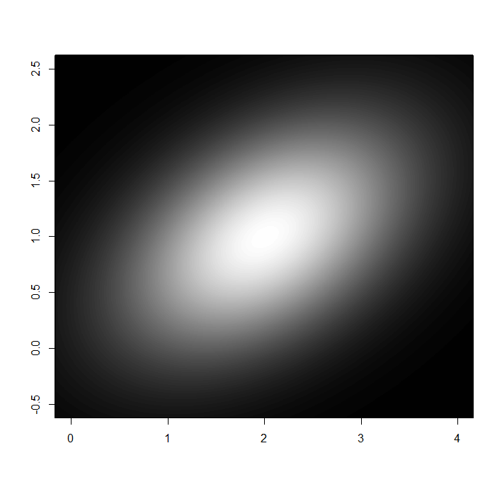
Figure 2
Figure 3 illustrates the process of computing \(\Pr\left(2<X_{1}<4,\,1<X_{2}<2\right)\) when \(X_{1}\) and \(X_{2}\) have the above joint density, using \(N_{1}=8\) and \(N_{2}=5\).
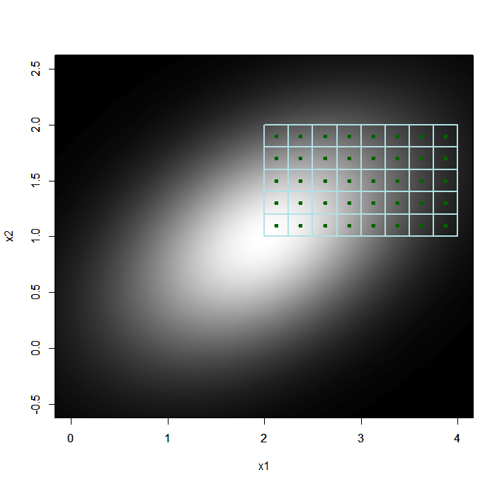
Figure 3
We can, of course, generalize this to joint distributions over three, four, or more variables \(X_{1},\ldots,X_{n}\), with a corresponding joint probability density function \(f\left(x_{1},\ldots,x_{n}\right)\). If \(a_{1}<b_{1}\) and … and \(a_{n}<b_{n}\), then the probability that \(a_{1}<X_{1}<b_{1}\) and … and \(a_{n}<X_{n}<b_{n}\) is the nested integral
\(\displaystyle \Pr\left(a_{1}<X_{1}<b_{1},\ldots,a_{n}<X_{n}<b_{n}\right)=\int_{a_{1}}^{b_{1}}\cdots\int_{a_{n}}^{b_{n}}f\left(x_{1},\ldots,x_{n}\right)\,\mathrm{d}x_{n}\,\cdots\,\mathrm{d}x_{1} \)
and we can think of this as choosing very large numbers \(N_{1},\ldots,N_{n}\) and forming an \(n\)-dimensional grid with \(N_{1}\times\cdots\times N_{n}\) cells, evaluating \(f\left(x_{1},\ldots,x_{n}\right)\) at the midpoint of each of these cells, and so on.
Conditional probability densities
Suppose that we have variables \(X_{1}\) and \(X_{2}\) with a joint distribution that has density function \(f\left(x_{1},x_{2}\right)\), describing our prior information about \(X_{1}\) and \(X_{2}\). We then find out the value of \(X_{1}\), perhaps via some sort of a measurement. Our updated information about \(X_{2}\) is summarized in the conditional distribution for \(X_{2}\), given that \(X_{1}=x_{1}\); the density function for this conditional distribution is
\(\displaystyle f\left(x_{2}\mid x_{1}\right)=\frac{f\left(x_{1},x_{2}\right)}{\int_{-\infty}^{\infty}f\left(x_{1},x_{2}\right)\,\mathrm{d}x_{1}}. \)
For example, if \(X_{1}\) and \(X_{2}\) have the joint distribution described in Figure 3, then Figure 4 shows the conditional density function for \(X_{2}\) given \(X_{1}=1\), and Figure 5 shows the conditional density function for \(X_{2}\) given \(X_{1}=3\). You can see from the density plot that \(X_{1}\) and \(X_{2}\) are positively correlated, and this explains why the density curve for \(X_{2}\) given \(X_{1}=3\) is shifted to the right relative to the density curve for \(X_{2}\) given \(X_{1}=1\).

Figure 4

Figure 5
In general, if we have joint probability distribution for \(n\) variables \(X_{1},\ldots,X_{n}\), with a joint probability density function \(f\left(x_{1},\ldots,x_{n}\right)\), and we find out the values of, say, \(X_{m+1},\ldots,X_{n}\), then we write
\(\displaystyle f\left(x_{1},\ldots,x_{m}\mid x_{m+1},\ldots,x_{n}\right) \)
for the conditional density function for \(X_{1},\ldots,X_{m}\), given that \(X_{m+1}=x_{m+1},\ldots,X_{n}=x_{n}\), and its formula is
\(\displaystyle f\left(x_{1},\ldots,x_{m}\mid x_{m+1},\ldots,x_{n}\right)=\frac{f\left(x_{1},\ldots,x_{n}\right)}{\int_{-\infty}^{\infty}\cdots\int_{-\infty}^{\infty}f\left(x_{1},\ldots,x_{n}\right)\,\mathrm{d}x_{m+1}\,\cdots\,\mathrm{d}x_{n}}. \)
One way of understanding this formula is to realize that if you integrate the conditional density over all possible values of \(X_{1},\ldots,X_{n}\), the result must be 1 (one of those possible values must be the actual value), and this is what the denominator in the above formula guarantees.
Change of variables
Suppose that we have two variables \(x\) and \(y\) that have a known deterministic relation that allows us to always obtain the value of \(y\) from the value of \(x\), and likewise obtain the value of \(x\) from the value of \(y\). Some examples are
- \(y=2x\) and \(x=\frac{1}{2}y\),
- \(y=e^{x}\) and \(x=\ln(y)\), or
- \(y=x^{3}\) and \(x=y^{1/3}\),
but not \(y=x^{2}\) when \(x\) may be positive or negative: if we are given \(y\) then \(x\) could be either \(+\sqrt{y}\) or \(-\sqrt{y}\).
If we have a probability density \(f_{\mathrm{y}}\) for \(y\) then we can turn it into a probability density \(f_{\mathrm{x}}\) for \(x\) using the change of variables formula:
\(\displaystyle f_{\mathrm{x}}(x)=f_{\mathrm{y}}(y)\left|\frac{\mathrm{d}y}{\mathrm{d}x}\right|. \)
In the above formula, \(\mathrm{d}y/\mathrm{d}x\) stands for the derivative of \(y\) with respect to \(x\); this measures how much \(y\) changes relative to a change in \(x\), and in general it depends on \(x\). Loosely speaking, imagine changing \(x\) by a vanishingly small amount \(\mathrm{d}x\), and let \(\mathrm{d}y\) be the corresponding (vanishingly small) change in \(y\); then the derivative of \(y\) with respect to \(x\) is the ratio \(\mathrm{d}y/\mathrm{d}x\).
Here are some common changes of variable:
- \(y=a\,x\) where \(a\) is some nonzero constant. Then
\(\displaystyle \begin{eqnarray*} \frac{\mathrm{d}y}{\mathrm{d}x} & = & a\\ f_{\mathrm{x}}(x) & = & a\,f_{\mathrm{y}}(y)\\ & = & a\,f_{\mathrm{y}}(ax). \end{eqnarray*}\)
- \(y=e^{x}\). Then
\(\displaystyle \begin{eqnarray*} \frac{\mathrm{d}y}{\mathrm{d}x} & = & y\\ f_{\mathrm{x}}(x) & = & y\,f_{\mathrm{y}}(y)\\ & = & e^{x}\,f_{\mathrm{y}}\left(e^{x}\right) \end{eqnarray*}\)
- \(y=\mathrm{logit}(x)=\ln(x/(1-x))\), where \(0<x<1\). Then
\(\displaystyle \begin{eqnarray*} \frac{\mathrm{d}y}{\mathrm{d}x} & = & \frac{1}{x\,(1-x)}\\ f_{\mathrm{x}}(x) & = & \frac{f_{\mathrm{y}}(y)}{x\,(1-x)}\\ & = & \frac{f_{\mathrm{y}}\left(\mathrm{logit}(x)\right)}{x\,(1-x)}. \end{eqnarray*}\)