(Part 1 is here.)

In part 1 I discussed choosing a sample size for the problem of inferring a proportion. Now, instead of a parameter estimation problem, let’s consider a hypothesis test.

This time we have two proportions \(\theta_0\) and \(\theta_1\), and two hypotheses that we want to compare: \(H_=\) is the hypothesis that \(\theta_0 = \theta_1\),  and \(H_{\ne}\) is the hypothesis that \(\theta_0 \ne \theta_1\). For example, we might be comparing the effects of a certain medical treatment and a placebo, with \(\theta_0\) being the proportion of patients who would recover if given the placebo, and \(\theta_1\) being the proportion of patients who would recover if given the medical treatment.

To fully specify the two hypotheses we must define their priors for \(\theta_0\) and \(\theta_1\). For appropriate values \(\alpha > 0\) and \(\beta > 0\) let us define

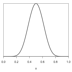
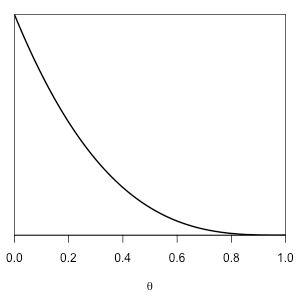
• \(H_=\): \(\theta_0 \sim \mathrm{beta}(\alpha,\beta)\) and \(\theta_1 = \theta_0\).
• \(H_{\ne}\): \(\theta_0 \sim \mathrm{beta}(\alpha, \beta)\)  and \(\theta_1 \sim \mathrm{beta}(\alpha, \beta)\) independently.

(\(\mathrm{beta}(\alpha,\beta)\) is a beta distribution over the interval \((0,1)\).) Our data are

• \(n_0\) and \(k_0\): the number of trials in population 0 and the number of positive outcomes among these trials.
• \(n_1\) and \(k_1\): the number of trials in population 1 and the number of positive outcomes among these trials.

We also define \(n = n_0 + n_1\) and \(k = k_0 + k_1\).

To get the likelihood of the data conditional only on the hypothesis \(H_=\) or \(H_{\ne}\) itself, without specifying a particular value for the parameters \(\theta_0\) or \(\theta_1\), we must “sum” (or rather, integrate) over all possible values of the parameters. This is called the marginal likelihood. In particular, the marginal likelihood of \(H_=\) is

\( \displaystyle \begin{aligned} & \Pr(k_0, k_1 \mid n_0, n_1, H_=)  \\ = &  \int_0^1 \mathrm{beta}(\theta \mid \alpha, \beta)\, \Pr\left(k_0 \mid n_0, \theta\right) \, \Pr\left(k_1 \mid n_0,\theta\right) \,\mathrm{d}\theta  \\ = &  c_0 c_1 \frac{\mathrm{B}(\alpha + k, \beta + n – k)}{\mathrm{B}(\alpha, \beta)} \end{aligned} \)

where \(\mathrm{B}\) is the beta function (not the beta distribution) and

\(\displaystyle \begin{aligned}c_0 & = \binom{n_0}{k_0} \\ c_1 & = \binom{n_1}{k_1} \\ \Pr\left(k_i\mid n_i,\theta\right) & = c_i \theta^{k_i} (1-\theta)^{n_i-k_i}. \end{aligned} \)

The marginal likelihood of \(H_{\ne}\) is

\( \displaystyle \begin{aligned} & \Pr\left(k_0, k_1 \mid n_0, n_1, H_{\ne}\right) \\ = & \int_0^1\mathrm{beta}\left(\theta_0 \mid \alpha, \beta \right)\, \Pr\left(k_0 \mid n_0, \theta_0 \right) \,\mathrm{d}\theta_0\cdot \\ & \int_0^1 \mathrm{beta}\left(\theta_1 \mid \alpha, \beta \right) \, \Pr\left(k_1 \mid n_1, \theta_1 \right)\,\mathrm{d}\theta_1 \\ = & c_0 \frac{\mathrm{B}\left(\alpha + k_0, \beta + n_0 – k_0\right)}{\mathrm{B}(\alpha, \beta)} \cdot  c_1 \frac{\mathrm{B}\left(\alpha + k_1, \beta + n_1 – k_1\right)}{\mathrm{B}(\alpha, \beta)}. \end{aligned} \)

Writing \(\Pr\left(H_=\right)\) and \(\Pr\left(H_{\ne}\right)\) for the prior probabilities we assign to \(H_=\) and \(H_{\ne}\) respectively, Bayes’ rule tells us that the posterior odds for \(H_=\) versus \(H_{\ne}\) is

\(\displaystyle \begin{aligned}\frac{\Pr\left(H_= \mid n_0, k_0, n_1, k_1\right)}{ \Pr\left(H_{\ne} \mid n_0, k_0, n_1, k_1\right)} & = \frac{\Pr\left(H_=\right)}{\Pr\left(H_{\ne}\right)} \cdot \frac{\mathrm{B}(\alpha, \beta)  \mathrm{B}(\alpha + k, \beta + n – k)}{ \mathrm{B}\left(\alpha + k_0, \beta + n_0 – k_0\right)  \mathrm{B}\left(\alpha + k_1, \beta + n_1 – k_1\right)}. \end{aligned} \)

Defining \(\mathrm{prior.odds} = \Pr\left(H_{=}\right) / \Pr\left(H_{\ne}\right)\), the following R code computes the posterior odds:

post.odds <- function(prior.odds, α, β, n0, k0, n1, k1) {
  n <- n0 + n1
  k <- k0 + k1
  exp(
    log(prior.odds) +
    lbeta(α, β) + lbeta(α + k, β + n - k) -
    lbeta(α + k0, β + n0 - k0) - lbeta(α + k1, β + n1 - k1))
}

We want the posterior odds to be either very high or very low, corresponding to high confidence that \(H_=\) is true or high confidence that \(H_{\ne}\) is true, so let’s choose as our quality criterion the expected value of the smaller of the posterior odds and its inverse:

$$ E\left[\min\left(\mathrm{post.odds}\left(k_0,k_1\right), 1/\mathrm{post.odds}\left(k_0,k_1\right)\right) \mid n_0, n_1, \alpha, \beta \right] $$

where, for brevity, we have omitted the fixed arguments to \(\mathrm{post.odds}\). As before, this expectation is over the prior predictive distribution for \(k_0\) and \(k_1\).

In this case the prior predictive distribution does not have a simple closed form, and so we use a Monte Carlo procedure to approximate the expectation:

• For \(i\) ranging from \(1\) to \(N\),
  • Draw \(h=0\) with probability \(\Pr\left(H_=\right)\) or \(h=1\) with probability \(\Pr\left(H_{\ne}\right)\).
  • Draw \(\theta_0\) from the \(\mathrm{beta}(\alpha, \beta)\) distribution.
  • If \(h=0\) then set \(\theta_1 = \theta_0\); otherwise draw \(\theta_1\) from the \(\mathrm{beta}(\alpha, \beta)\) distribution.
  • Draw \(k_0\) from \(\mathrm{binomial}\left(n_0, \theta_0\right)\) and draw \(k_1\) from \(\mathrm{binomial}\left(n_1, \theta_1\right)\).
  • Define \(z = \mathrm{post.odds}\left(k_0, k_1\right)\).
  • Assign \(x_i = \min(z, 1/z)\).
• Return the average of the \(x_i\) values.

The following R code carries out this computation:

loss <- function(prior.odds, α, β, n0, k0, n1, k1) {
  z <- post.odds(prior.odds, α, β, n0, k0, n1, k1);
  pmin(z, 1/z)
}
expected.loss <- function(prior.odds, α, β, n0, n1) {
  # prior.odds = P.eq / P.ne = (1 - P.ne) / P.ne = 1/P.ne - 1
  # P.ne = 1 / (prior.odds + 1)
  N <- 1000000
  h <- rbinom(N, 1, 1 / (prior.odds + 1))
  θ0 <- rbeta(N, α, β)
  θ1 <- rbeta(N, α, β)
  θ1[h == 0] <- θ0[h == 0]
  k0 <- rbinom(N, n0, θ0)
  k1 <- rbinom(N, n1, θ1)
  x <- loss(prior.odds, α, β, n1, k1, n0, k0)
  # Return the Monte Carlo estimate +/- error estimate 
  list(estimate=mean(x), delta=sd(x)*1.96/sqrt(N))
}

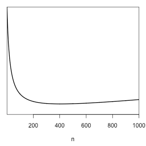
Suppose that \(H_=\) and \(H_{\ne}\) have equal prior probabilities, and \(\alpha=\beta=1\), that is, we have a uniform prior over \(\theta_0\) (and \(\theta_1\), if applicable). The following table shows the expected loss—the expected value of the minimum of the posterior odds against \(H_{\ne}\) and the posterior odds against \(H_=\)—as \(n_0 = n_1\) ranges from 200 to 1600:

\(n_0\)	\(n_1\)	Expected loss
200	200	0.130
400	400	0.095
600	600	0.078
800	800	0.069
1000	1000	0.062
1200	1200	0.057
1400	1400	0.053
1600	1600	0.050

We find that it takes 1600 trials from each population to achieve an expected posterior odds in favor of the (posterior) most probable results of 20 to 1.

I recently encountered a claim that Bayesian methods could provide no guide to the task of estimating what sample size an experiment needs in order to reach a desired level of confidence. The claim was as follows:

1. Bayesian theory would have you run your experiment indefinitely, constantly updating your beliefs.
2. Pragmatically, you have resource limits so you must determine how best to use those limited resources.
3. Your only option is to use frequentist methods to determine how large of a sample you’ll need, and then to use frequentist methods to analyze your data.

(2) above is correct, but (1) and (3) are false. Bayesian theory allows you to run your experiment indefinitely, but in no way requires this. And Bayesian methods not only allow you to determine a required sample size, they are also far more flexible than frequentist methods in this regard.

For concreteness, let’s consider the problem of estimating a proportion:

• We have a parameter \(\theta\), \(0 \leq \theta \leq 1\), which is the proportion to estimate.
• We run an experiment \(n\) times, and \(x_i\), \(1 \leq i \leq n\) is the outcome of experiment \(i\). This outcome may be 0 or 1.
• Our statistical model is \(x_i \sim \mathrm{Bernoulli}(\theta) \) for all \(1 \leq i \leq n\), that is,
  • \(x_i = 1\) with probability \(\theta\),
  • \(x_i = 0\) with probability \(1-\theta\), and
  • \(x_i\) and \(x_j\) are independent for \(i \ne j\).
• We are interested in the width \(w\) of the 95% posterior credible interval for \(\theta\).

For example, we could be running an opinion poll in a large population, with \(x_i\) indicating an answer of yes=1 or no=0 to a survey question. Each “experiment” is an instance of getting an answer from a random survey respondent, \(n\) is the number of people surveyed, and \(k\) is the number of “yes” answers.

We’ll use a \(\mathrm{beta}(\alpha,\beta)\) prior \((\alpha,\beta>0)\) to describe our prior information about \(\theta\). This is a distribution over the interval \([0,1]\) with mean \(\alpha/\beta\) and a shape determined by \(\alpha\); higher values of \(\alpha\) correspond to more sharply concentrated distributions.

If \(\alpha=\beta=1\) then we have a uniform distribution over \([0,1]\). If \(\alpha=\beta=10\) then \(\mathrm{beta}(\alpha,\beta)\) is the following distribution with mean 0.5:

 

Such a prior might be appropriate, for example, for an opinion poll on a topic for which you expect to see considerable disagreement.

If \(\alpha=1,\beta=4\) then \(\mathrm{beta}(\alpha,\beta)\) is the following distribution with mean 0.2:

If we have \(k\) positive outcomes out of \(n\) trials, then our posterior distribution for \(\theta\) is \(\mathrm{beta}(\alpha+k,\beta+n-k)\), and the 95% equal-tailed posterior credible interval is the difference between the 0.975 and 0.025 quantiles of this distribution; we compute this in R as

w <- qbeta(.975, α + k, β + n - k) - qbeta(.025, α + k, β + n - k)

If you prefer to think in terms of \(\hat{\theta}\pm\Delta\), a point estimate \(\hat{\theta}\) plus or minus an error width \(\Delta\), then choosing \(\hat{\theta}\) to be the midpoint of the 95% credible interval gives \(\Delta=w/2\).

Note that \(w\) depends on both \(n\), the number of trials, and \(k\), the number of positive outcomes we observe; hence we write \(w = w(n,k)\). Although we may choose \(n\) in advance, we do not know what \(k\) will be. However, combining the prior for \(\theta\) with the distribution for \(k\) conditional on \(n\) and \(\theta\) gives us a prior predictive distribution for \(k\):

$$ \Pr(k \mid n) = \int_0^1\Pr(k \mid n,\theta) \mathrm{beta}(\theta \mid \alpha, \beta)\,\mathrm{d}\theta. $$

\(\Pr(k \mid n, \theta)\) is a binomial distribution, and the prior predictive distribution \(\Pr(k \mid n)\) is a weighted average of the binomial distributions for \(k\) you get for different values of \(\theta\), with the prior density serving as the weighting. This weighted average of binomial distributions is known as the beta-binomial distribution \(\mathrm{betabinom}(n,\alpha,\beta)\).

So we use as our quality criterion \(E[w(n,k) \mid n, \alpha, \beta]\), the expected value of the posterior credible interval width \(w\), using the prior predictive distribution \(\mathrm{betabinom}(n,\alpha,\beta)\) for \(k\).  The file edcode1.R contains R code to compute this expected posterior width for arbitrary choices of \(n\), \(\alpha\), and \(\beta\).

Here is a table of our quality criterior computed for various values of \(n\), \(\alpha\), and \(\beta\):

\(n\)	\(\alpha\)	\(\beta\)	\(E[w(n,k)\mid n,\alpha,\beta]\)	\(E[\Delta(n,k)\mid n,\alpha,\beta]\)
100	1	1	0.152	0.076
200	1	1	0.108	0.054
300	1	1	0.089	0.044
100	10	10	0.174	0.087
200	10	10	0.129	0.064
300	10	10	0.107	0.053
100	1	4	0.131	0.066
200	1	4	0.094	0.047
300	1	4	0.077	0.039

We could then create a table such as this and choose a value for \(n\) that gave an acceptable expected posterior width. But we can do so much more…

This problem is a decision problem, and hence the methods of decision analysis are applicable here. The Von Neumann – Morgenstern utility theorem tells us that any rational agent make its choices as if it were maximizing an expected utility function or, equivalently, minimizing an expected loss function. For this problem, we can assume that

• The cost of the overall experiment increases as \( n \) increases; thus our loss function increases with \( n \).
• We prefer knowing \( \theta \) with more certainty over knowing it with less certainty; thus our loss function increases with \( w \), where \( w \) is the width of the 95% credible interval for \( \theta \).

This suggests a loss function of the form

$$ L(n, w) = f(n) + g(w) $$

where \(f\) and \(g\) are strictly increasing functions. If we must choose \(n\) in advance, then we should choose it so as to minimize the expected loss

$$ E[L(n,w)] = f(n) + E[g(w)]. $$

which we can compute via a slight modification to the code in edcode1.R:

expected.loss <- function(α, β, n) {
  f(n) + sum(dbetabinom.ab(0:n, n, α, β) * g(posterior.width(α, β, n, 0:n)))
}

For example, suppose that this is a survey. If each response costs us $2, then \(f(n)=2n\). Suppose that \(g(w)=10^5w^2\), i.e., we would be willing to pay \(10^5(0.10)^2 – 10^5(0.05)^2\) or $750 to decrease the posterior width from 0.10 to 0.05. If a \(\mathrm{beta}(10,10)\) distribution describes our prior information, then the following plot shows the expected loss for \(n\) ranging from 1 to 1000,

and \(n=407\) is the optimal choice.

This is a topic I just have to comment on, given the recent movie Noah and some comments I have heard from family members. I find it astounding that an educated, intelligent person, especially one with a degree in engineering or a hard science, could believe that the story of Noah and the Flood in Genesis is a literal, historical account. The only evidence in favor of it is an ancient legend recounted in the Bible and the story of Gilgamesh.  Everything else argues against it. This is not a question of just one or two anomalies; the story falls to pieces pretty much however you approach it.

Others have already gone over this ground in detail, so I’ll just link to one of these articles—The Impossible Voyage of Noah’s Ark—and mention a few obvious problems that occur to me.

First, let’s talk prior plausibility.

How plausible is it that a construction crew of at most 8 people could build a wooden vessel much larger than any ever constructed in the 4500 years since, using pre-industrial, Bronze Age technology?

Assuming an 18-inch cubit, the Bible claims that the ark measured 450 feet long, 75 feet wide, and 45 feet high, that it was made out of “gopher wood,” and that it was sealed with pitch, presumably to keep it water tight. The ark as described in the Bible is essentially a barge, so I did a quick web search on the largest wooden ships ever built, and the closest thing I could find to the claimed size of Noah’s ark was the Pretoria, a huge barge built in 1900.

At the time of its construction, the Pretoria was the largest wooden ship that had ever been built, and is nearly the largest wooden ship of any kind ever built. Nevertheless, the Pretoria measured considerably smaller than the claimed dimensions of Noah’s ark: 338 feet long, 44 feet wide wide, and 23 feet in depth, or just under 1/4 the claimed total volume for Noah’s ark. Like other such large wooden ships, the Pretoria’s frame and hull required strengthening with steel plates and bands, along with a steam engine to pump out the water that leaked in. According to the 1918 book How Wooden Ships Are Built (by Harvey Cole Estep), “If current practice is any guide, it may safely be stated that steel reinforcement is necessary for hulls over 275 feet in length and exceeding, say, 3500 tons dead weight.”

Then there’s the question of where all that water came from, and where it went. A simple calculation shows that it would require about an additional 4.5 billion cubic kilometers of water to cover the whole Earth up to the top of Mount Everest, or nearly 3-1/2 times the current total volume of the world’s oceans. If you want to hypothesize that somehow such high mountains didn’t exist prior to the Flood, and were raised up afterwards, then you have several severe problems:

• Every time you add a new ad hoc addendum to your hypothesis to patch up a hole in the story, this as a logical necessity lowers the prior probability of the overall scenario.
• The best geological evidence says that the Himalayas are about 50 million years old. They were definitely around at the time of the presumed Flood.
• If you want to argue, against the geologic evidence, that somehow the Himalayas weren’t raised up until after 2500 B.C., consider the energies involved! If you want to raise up the Himalayas in at most a few hundred years, instead over 50 million years, you are talking continual, massive earthquakes for that entire period, and I’m guessing that the heat produced would melt a substantial portion of the Earth’s crust.

Second, let’s consider expected consequences.

An obvious one is that archaeologists and paleontologists should be finding a very large number of scattered human and other animal skeletons all dating to the same time period of about 2500 B.C. Needless to say, they have found nothing like this.

There should be obvious signs in the geologic record of such a massive cataclysm, evidence that can be dated to about 4500 years ago. No such evidence exists.

The Bronze Age spans the years from 3300 B.C. to 1200 B.C. in the near East. See, for example, the Bronze Age article in the Ancient HIstory Encyclopedia. Do archaeologists find the civilizations of that era suddenly disappearing around 2500 B.C.? No, they do not.

Some fish live only in salt water, others only in fresh water. The flood described in the Bible would have either killed all of the salt-water fish (if the flood waters were fresh) or killed all of the fresh-water fish (if the flood waters were salty) or both (if the flood waters were of intermediate salinity).

What happens when you reduce an entire species down to a very small breeding population? Usually, it dies out—see the notion of a minimum viable population. But if the species avoids that fate, you get something like the cheetahs: an entire species whose members are all virtually identical genetic copies of each other. A world in which the Biblical Flood had really occurred would look very different from ours. Every animal species would consist entirely of near-identical duplicates. There would be no racial strife among humans, because we would all look nearly as alike as identical twins.

I’ve just scratched the surface here, without hardly trying. Anyone who actually sits down and thinks about it, and does a bit of honest research will have no trouble finding many more problems with the whole Flood story.

 

It is often claimed, with a triumphant air of finality, that “you can’t prove a negative.” Along similar lines it is often said, as if it were an unquestionable truth acknowledged by all, that “absence of evidence is not evidence of absence.”

Both of these supposed rules are epistemic nonsense.

You can prove that something doesn’t exist, and absence of some kinds of evidence is in fact evidence of absence. These are straightforward consequences of elementary probability theory.

Let’s first dispense with some obvious straw men. One might say, “Of course you can prove a negative; for example, it’s easy to prove that there does not exist any real number whose square is negative.” But that is a proof about the world of mathematical abstractions; when people say that you can’t prove a negative, they have in minding proving nonexistence of some entity or phenomenon in the physical world. This is the more interesting case that I am addressing here.

The second straw man goes in the other direction: it is true, in a vacuous and utterly uninteresting sense, that you can’t prove nonexistence of a hypothesized phenomenon or entity with 100% certainty… but this is only true in the same sense that you can’t prove any claim about the physical world with 100% certainty. For example, I could claim that you are not actually reading these words, but are instead experiencing an elaborate hallucination as you drool in your padded cell in a mental institution. You cannot prove, with absolute certainty, that this is not the case. Absolute proof is reserved to the realm of mathematics only. In assessing claims about the physical world we are always working with imperfect information, and so the relevant question is not, can you prove that X is true, but rather, how probable is it that X is true?

So let’s agree that “prove,” in the context of assertions about the physical world, in practice means “demonstrate that a high degree of confidence is warranted.”

So how can you prove a negative, and how can you use absence of evidence as evidence of absence? The key lies in considering the probable consequences of a hypothesis. Consider the hypothesis, “There is a cat living in my apartment.” If this hypothesis is true, then I would expect to observe the following:

• Urine stains somewhere in the apartment; the cat has to pee sometime.
• Feces of a certain size appearing from time to time; the cat is going to have bowel movements.
• Food going missing; the cat has to eat sometime. Or, if the cat doesn’t eat, it’s going to die, and I expect the bad smell of a decomposing body to eventually become evident.
• Scratched up furniture or other items; it’s an established behavioral pattern of cats that they scratch things.
• Unexplained sounds of movement. It’s unlikely that the cat can be so thoroughly stealthy that, aside from never seeing it, I never even hear it.
• Loose animal hairs on the carpet or in other areas around the apartment.
• Sneezing, itching, and a runny nose even when I’m not suffering a cold and it’s not allergy season. (I’m allergic to cat dander.)

If I observe none of these expected consequences of a cat living in my apartment, I can be very confident that there is, in fact, no cat living in my apartment. I have proven a negative through a lack of evidence.

Notice the form of this logical rule: absence of expected evidence is evidence of absence. If I did not expect to have this evidence—say, because I haven’t even entered the apartment for the last three months—then its absence would be meaningless.

For an entertaining fictional illustration of this idea, let’s look at the Sherlock Holmes story, “Silver Blaze.” A race horse has been stolen and its trainer killed. Suspicion is laid upon a man named Fitzroy Simpson. Holmes argues that Simpson could have been present in the stables that night:

Gregory (Scotland Yard detective): “Is there any other point to which you would wish to draw my attention?”

Holmes: “To the curious incident of the dog in the night-time.”

Gregory: “The dog did nothing in the night-time.”

Holmes: “That was the curious incident.”

As Holmes later explained,

…a dog was kept in the stables, and yet, though some one had been in and fetched out a horse, he had not barked enough to arouse the two lads in the loft. Obviously the midnight visitor was some one whom the dog knew well.

(You can stop here if the above intuitive explanation satisfies you.) Here’s the math, for those who are interested:

$$ \frac{\Pr(A \mid \neg D, X)}{\Pr(\neg A \mid \neg D,X)} = \frac{\Pr(A \mid X)}{\Pr(\neg A \mid X)} \cdot \frac{\Pr(\neg D \mid A, X)}{\Pr(\neg D \mid \neg A, X)} $$

In the above equation,

• \(X\) stands for any relevant background information;
• \(A\) stands for the hypothesis and \(\neg A\) stands for its negation (the statement that the hypothesis is false);
• \(D\) stands for a datum that is not observed;
• \(\Pr(A \mid X)\) means the probability of hypothesis \(A\) given only the background information \(X\), and similarly for the other expressions of the same form.

In the example of the cat, for the specific expected evidence of urine stains, we would have the following:

• \(A\) means “there is a cat living in my apartment.”
• \(\neg A\) means “there is not a cat living in my apartment.”
• \(D\) means “I find urine stains in the apartment.”
• \(\neg D\) means “I do not find urine stains in the apartment.”
• \(X\) might stand for background information such as “I have never brought a cat into the apartment.”
• \(\Pr(A \mid \neg D, X)\) means “the probability that there is a cat living in my apartment, given that I find no urine stains in the apartment and I have never brought a cat into the apartment.”
• \(\Pr(\neg A \mid \neg D, X)\) means “the probability that there is not a cat living in my apartment, given that I find no urine stains in the apartment and I have never brought a cat into the apartment.”
• The expression $$ \frac{\Pr(A \mid \neg D, X)}{\Pr(\neg A \mid \neg D, X)} $$ is the odds in favor of there being a cat living in my apartment, given that I find no urine stains and have never brought a cat into the apartment.
• \(\Pr(A \mid X)\) means “the probability that there is a cat living in my apartment, given that I have never brought a cat into the apartment”.
• \(\Pr(\neg A \mid X)\) means “the probability that there is not a cat living in my apartment, given that I have never brought a cat into the apartment”.
• The expression $$ \frac{\Pr(A \mid X)}{\Pr(\neg A \mid X)} $$ is the odds in favor of there being a cat living in my apartment, given only the information that I have never brought a cat into the apartment.
• \(\Pr(D \mid A, X)\) means “the probability that I find urine stains in my apartment, if there is a cat living in my apartment and I have never brought a cat into my apartment.”
• \(\Pr(D \mid \neg A,X\) means “the probability that I find urine stains in my apartment, if there is not a cat living in my apartment and I have never brought a cat into my apartment.”
• The expression $$ \frac{\Pr(\neg D \mid A, X)}{\Pr(\neg D \mid \neg A, X)} $$ is the likelihood ratio for the (lack of) evidence; that is, the ratio of (a) the probability that I find no urine stains if there is a cat living in my apartment, versus (b) the probability that I find no urine stains if there is not a cat living in my apartment.

The important point is that $$ \Pr(\neg D \mid A, X) < \Pr(\neg D \mid \neg A, X). $$ That is, it is more probable that I find no urine stains if there is no cat living in my apartment than it is to find no urine stains if there is a cat living in my apartment. The fact that I do not find urine stains in my apartment multiplies the initial odds in favor of there being a cat living in my apartment by a number less than one, thus decreasing those odds. Each additional piece of expected evidence that I do not find further decreases the odds.