
I recently encountered a claim that Bayesian methods could provide no guide to the task of estimating what sample size an experiment needs in order to reach a desired level of confidence. The claim was as follows:
- Bayesian theory would have you run your experiment indefinitely, constantly updating your beliefs.
- Pragmatically, you have resource limits so you must determine how best to use those limited resources.
- Your only option is to use frequentist methods to determine how large of a sample you’ll need, and then to use frequentist methods to analyze your data.
(2) above is correct, but (1) and (3) are false. Bayesian theory allows you to run your experiment indefinitely, but in no way requires this. And Bayesian methods not only allow you to determine a required sample size, they are also far more flexible than frequentist methods in this regard.
For concreteness, let’s consider the problem of estimating a proportion:
- We have a parameter \(\theta\), \(0 \leq \theta \leq 1\), which is the proportion to estimate.
- We run an experiment \(n\) times, and \(x_i\), \(1 \leq i \leq n\) is the outcome of experiment \(i\). This outcome may be 0 or 1.
- Our statistical model is \(x_i \sim \mathrm{Bernoulli}(\theta) \) for all \(1 \leq i \leq n\), that is,
- \(x_i = 1\) with probability \(\theta\),
- \(x_i = 0\) with probability \(1-\theta\), and
- \(x_i\) and \(x_j\) are independent for \(i \ne j\).
- We are interested in the width \(w\) of the 95% posterior credible interval for \(\theta\).
For example, we could be running an opinion poll in a large population, with \(x_i\) indicating an answer of yes=1 or no=0 to a survey question. Each “experiment” is an instance of getting an answer from a random survey respondent, \(n\) is the number of people surveyed, and \(k\) is the number of “yes” answers.
We’ll use a \(\mathrm{beta}(\alpha,\beta)\) prior \((\alpha,\beta>0)\) to describe our prior information about \(\theta\). This is a distribution over the interval \([0,1]\) with mean \(\alpha/\beta\) and a shape determined by \(\alpha\); higher values of \(\alpha\) correspond to more sharply concentrated distributions.
If \(\alpha=\beta=1\) then we have a uniform distribution over \([0,1]\). If \(\alpha=\beta=10\) then \(\mathrm{beta}(\alpha,\beta)\) is the following distribution with mean 0.5:
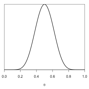
Such a prior might be appropriate, for example, for an opinion poll on a topic for which you expect to see considerable disagreement.
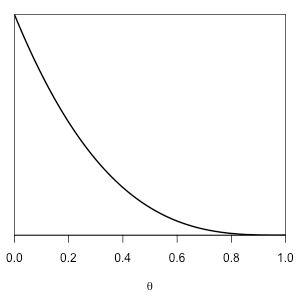
If \(\alpha=1,\beta=4\) then \(\mathrm{beta}(\alpha,\beta)\) is the following distribution with mean 0.2:
If we have \(k\) positive outcomes out of \(n\) trials, then our posterior distribution for \(\theta\) is \(\mathrm{beta}(\alpha+k,\beta+n-k)\), and the 95% equal-tailed posterior credible interval is the difference between the 0.975 and 0.025 quantiles of this distribution; we compute this in R as
w <- qbeta(.975, α + k, β + n - k) - qbeta(.025, α + k, β + n - k)
If you prefer to think in terms of \(\hat{\theta}\pm\Delta\), a point estimate \(\hat{\theta}\) plus or minus an error width \(\Delta\), then choosing \(\hat{\theta}\) to be the midpoint of the 95% credible interval gives \(\Delta=w/2\).
Note that \(w\) depends on both \(n\), the number of trials, and \(k\), the number of positive outcomes we observe; hence we write \(w = w(n,k)\). Although we may choose \(n\) in advance, we do not know what \(k\) will be. However, combining the prior for \(\theta\) with the distribution for \(k\) conditional on \(n\) and \(\theta\) gives us a prior predictive distribution for \(k\):
$$ \Pr(k \mid n) = \int_0^1\Pr(k \mid n,\theta) \mathrm{beta}(\theta \mid \alpha, \beta)\,\mathrm{d}\theta. $$
\(\Pr(k \mid n, \theta)\) is a binomial distribution, and the prior predictive distribution \(\Pr(k \mid n)\) is a weighted average of the binomial distributions for \(k\) you get for different values of \(\theta\), with the prior density serving as the weighting. This weighted average of binomial distributions is known as the beta-binomial distribution \(\mathrm{betabinom}(n,\alpha,\beta)\).
So we use as our quality criterion \(E[w(n,k) \mid n, \alpha, \beta]\), the expected value of the posterior credible interval width \(w\), using the prior predictive distribution \(\mathrm{betabinom}(n,\alpha,\beta)\) for \(k\). The file edcode1.R contains R code to compute this expected posterior width for arbitrary choices of \(n\), \(\alpha\), and \(\beta\).
Here is a table of our quality criterior computed for various values of \(n\), \(\alpha\), and \(\beta\):
| \(n\) | \(\alpha\) | \(\beta\) | \(E[w(n,k)\mid n,\alpha,\beta]\) | \(E[\Delta(n,k)\mid n,\alpha,\beta]\) |
|---|---|---|---|---|
| 100 | 1 | 1 | 0.152 | 0.076 |
| 200 | 1 | 1 | 0.108 | 0.054 |
| 300 | 1 | 1 | 0.089 | 0.044 |
| 100 | 10 | 10 | 0.174 | 0.087 |
| 200 | 10 | 10 | 0.129 | 0.064 |
| 300 | 10 | 10 | 0.107 | 0.053 |
| 100 | 1 | 4 | 0.131 | 0.066 |
| 200 | 1 | 4 | 0.094 | 0.047 |
| 300 | 1 | 4 | 0.077 | 0.039 |
We could then create a table such as this and choose a value for \(n\) that gave an acceptable expected posterior width. But we can do so much more…
This problem is a decision problem, and hence the methods of decision analysis are applicable here. The Von Neumann – Morgenstern utility theorem tells us that any rational agent make its choices as if it were maximizing an expected utility function or, equivalently, minimizing an expected loss function. For this problem, we can assume that
- The cost of the overall experiment increases as \( n \) increases; thus our loss function increases with \( n \).
- We prefer knowing \( \theta \) with more certainty over knowing it with less certainty; thus our loss function increases with \( w \), where \( w \) is the width of the 95% credible interval for \( \theta \).
This suggests a loss function of the form
$$ L(n, w) = f(n) + g(w) $$
where \(f\) and \(g\) are strictly increasing functions. If we must choose \(n\) in advance, then we should choose it so as to minimize the expected loss
$$ E[L(n,w)] = f(n) + E[g(w)]. $$
which we can compute via a slight modification to the code in edcode1.R:
expected.loss <- function(α, β, n) {
  f(n) + sum(dbetabinom.ab(0:n, n, α, β) * g(posterior.width(α, β, n, 0:n)))
}
For example, suppose that this is a survey. If each response costs us $2, then \(f(n)=2n\). Suppose that \(g(w)=10^5w^2\), i.e., we would be willing to pay \(10^5(0.10)^2 – 10^5(0.05)^2\) or $750 to decrease the posterior width from 0.10 to 0.05. If a \(\mathrm{beta}(10,10)\) distribution describes our prior information, then the following plot shows the expected loss for \(n\) ranging from 1 to 1000,
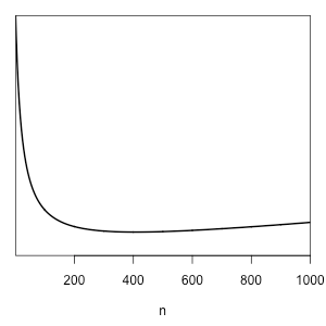 and \(n=407\) is the optimal choice.